
Contents | 1. Introduction to structural design |
Introduction to loads | Dead loads | Live loads |
Environmental loads are those due to snow, wind, rain, soil (and hydrostatic pressure) and earthquake. Unlike live loads, which are assumed to act on all floor surfaces equally, independent of the geometry or material properties of the structure, most of these environmental loads depend not only upon the environmental processes responsible for producing the loads, but upon the geometry or weight of the building itself. For snow, wind and earthquake loads, the "global" environmental considerations can be summarized by location-dependent numbers for each phenomenon: ground snow load for snow, basic wind speed for wind, and maximum ground motion (acceleration) for earthquake (Appendix Table A-2.3). Considerations specific to each building are then combined with these "global" environmental numbers to establish the magnitude and direction of forces expected to act on the building. Like live loads, the actual procedures for calculating environmental loads are not derived independently for each building, but are mandated by local building codes. For the actual design of real buildings in real places, the governing building code must be consulted; for the preliminary design of real or imaginary buildings, the following guidelines will do.
Determining the weight of snow that might fall on a structure starts with a ground snow load map, or a ground snow load value determined by a local building code official. These values range from zero to 100 psf for most regions, although weights of up to 300 psf are possible in locations such as Whittier, Alaska. Some typical ground snow load values are listed in Appendix Table A-2.3. Flat roof snow loads are generally considered to be about 30% less than these ground snow load values, and both wind and thermal effects — as well as the "importance" of the structure — are accounted for in further modifying this roof load. A thermal factor, Ct = 1.2, is included in the flat roof load for unheated structures (Ct = 1.0 for heated structures and 1.1 for heated structures with ventilated roofs protected with at least R-25 insulation below the ventilated plenum or attic); we will assume a nominal value of 1.0 for both wind ("exposure") and "importance." Other possible values for the snow load importance factor, Is, are listed in Appendix Table A-2.4. However, the major parameter in determining snow loads is the slope of the surface expected to carry the load. As the slope increases, more snow can be expected to slide off the roof surface, especially if the surface is slippery, and if the space immediately below the surface is heated. The slope-reduction factor, CS, which is multiplied by the flat roof snow load to obtain the actual roof snow load, takes these factors into account:
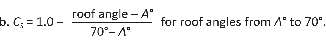
The parameter A (degrees Fahrenheit) depends on how slippery the roof surface is, and whether that surface is allowed to become warm or cold: A = 5° for warm, slippery roofs (where the R-value must be at least 30 for unventilated roofs, and at least 20 for ventilated roofs); 30° for warm, not slippery roofs (or for slippery roofs not meeting the R-value criteria); 15° for cold, slippery roofs; 45° for cold, not slippery roofs; and, for the intermediate condition where a roof remains somewhat cold because it is ventilated (with at least R-25 insulation below the ventilated space), A = 10° for slippery roofs; and 37.5° for not slippery roofs. Neglecting variations due to exposure, the snow load can be written as:
For low-slope roofs (i.e., hip, gable, or monoslope roofs with slopes less than 15°, the roof snow load cannot be taken less than Is × ground snow load or Is × 20 lb/ft2, whichever is less.
As an example, for "ordinary" buildings (Is = 1.0) with nonslippery (e.g., asphalt shingle) roofs having slopes no greater than 37.5°, kept cold by proper ventilation (with at least R-25 insulation below the ventilated space), the sloped roof snow load, deployed on the horizontal projection of the inclined structural roof members, becomes:
Judgment should be used where the building geometry provides opportunities for drifting snow to accumulate on lower roofs, or when sliding snow from higher roofs might fall on lower roofs. Most building codes provide guidelines for these situations.
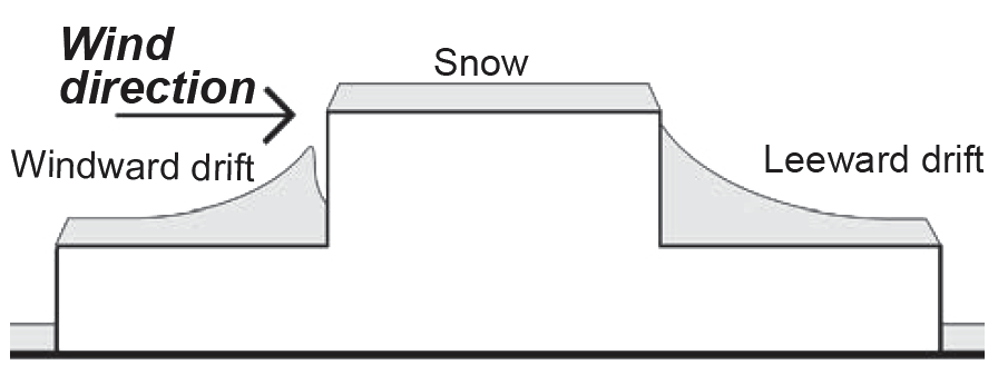
To account for the effects of wind acting simultaneously with snow on hip- or gable-type roofs, it is necessary to also check a so-called unbalanced snow load, caused by wind blowing snow from the windward to the leeward portion of the roof. In old building codes, this unbalanced load was computed by taking 1.5 times the snow load acting on the leeward side of the gable, with zero snow load on the windward side. Contemporary codes have a more complex strategy for computing such loads, but only applicable to hip and gable roofs with slopes between 2.38° (i.e., 1/2:12) and 30.26° (i.e., 7:12). Steeper or shallower roofs are not affected by wind-blown snow in the same way and so the calculation of such unbalanced loads is not required in these cases. For residential-scale buildings — i.e., where the horizontal distance from ridge to eave is not greater than 20 ft — the unbalanced snow load is taken as Is × ground snow load on the leeward side, with zero snow load on the windward side.
For larger buildings with ridge-to-eave horizontal distances greater than 20 ft, the unbalanced
snow load calculations are more easily performed using a spreadsheet or other software. A load
is first computed for the windward side, taken as 0.3 × roof snow load. In addition, there are two loads computed for the leeward side: the first is just the roof snow load taken over the entire leeward surface; the second has a magnitude of hdγ/![]() , but is placed on only part of the leeward roof, specifically, that rectangular portion on the leeward side extending from the ridge a distance, measured horizontally, of (8/3)hd
, but is placed on only part of the leeward roof, specifically, that rectangular portion on the leeward side extending from the ridge a distance, measured horizontally, of (8/3)hd![]() . In these calculations, hd (ft) is the height of a snow drift = 0.43(lu1/3)(ground snow load + 10)1/4 – 1.5; lu is the length of the roof upwind of the drift (ft), taken here as the horizontal distance from ridge to eave measured on the windward part of the roof; γ = the so-called snow density, taken as (0.13 × ground snow load) + 14 but no greater than 30 pcf; and S is a measure of the roof slope, taken as the horizontal run for a rise of 1.
. In these calculations, hd (ft) is the height of a snow drift = 0.43(lu1/3)(ground snow load + 10)1/4 – 1.5; lu is the length of the roof upwind of the drift (ft), taken here as the horizontal distance from ridge to eave measured on the windward part of the roof; γ = the so-called snow density, taken as (0.13 × ground snow load) + 14 but no greater than 30 pcf; and S is a measure of the roof slope, taken as the horizontal run for a rise of 1.
Two other circumstances may be of importance and require special consideration. First, where snow load is calculated on roofs or decks that are below the depth of the ground snow, the balanced snow load is taken as Is × ground snow load. Second, where a roof surface is adjacent to but below another roof surface, both the leeward and windward conditions must be considered, since either could create snow drifts on the lower roof, as shown schematically in Figure 2.10. Such calculations are rather complex and are not included here.
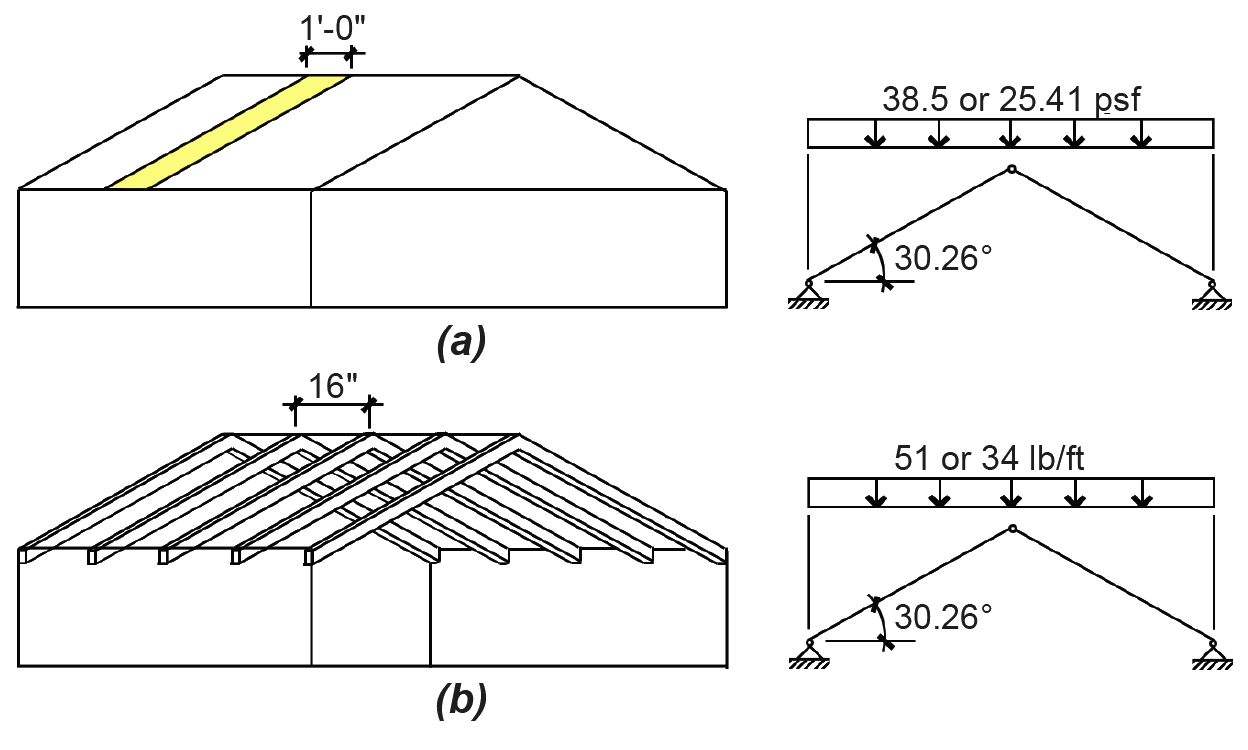
Problem definition. Find the snow load on a house in Portland, ME with a conventional roof with a 7:12 slope, i.e., with an angle = tan-1(7/12) = 30.26°. The roof is kept cold by having a ventilated attic, with R-30 insulation separating the ventilated attic space from the heated house below. Calculate for both asphalt shingles and metal roofing.
Solution overview. Solution overview. Find ground snow load; compute roof snow load.
Problem solution
1. From Appendix Table A-2.3, the ground snow load = 50 psf.
2. Find the roof snow load:
a. Nonslippery surface (asphalt shingles): From Equation 2.4, for this condition only, the snow load = 0.7(1.1)(1.0)(ground snow load) = 0.7(1.1)(1.0)(50) = 38.5 psf.
b. Slippery surface (metal roofing): From Equation 2.2, find the coefficient, CS for roof angles from A° to 70°, where A = 10° for cold, slippery roofs (kept cold by ventilation). In this case, CS = 1.0 – (roof angle – A°)/(70° – A°) = 1.0 – (30.26 – 10)/(70 – 10) = 0.66. From Equation 2.3, the snow load = 0.7CSCt(ground snow load) = 0.7(0.66)(1.1)(50) = 25.41 psf.
3. For rafters (sloped roof beams) spaced at 16 in. on center, the snow load on each rafter becomes:
a. 38.5(16/12) = 51 lb/ft for the non-slippery roof.
b. 25.41(16/12) = 34 lb/ft for the slippery roof.
4. Both of these loading diagrams are shown in Figure 2.11.
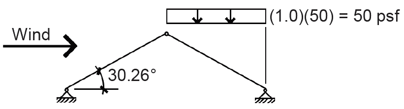
5. To account for the effects of wind acting simultaneously with snow on gable-type roofs, we also check the unbalanced snow load. Since the 30.26° slope of this roof falls between 2.38° and 30.26°, the unbalanced snow load on the leeward side must be computed. For residential-scale buildings — i.e., where the horizontal distance from ridge to eave is not greater than 20 ft — the unbalanced snow load is taken as Is × ground snow load, with zero snow load on the windward side. For this example, the unbalanced snow load diagram is shown in Figure 2.12.
Building codes take one of two approaches to the mathematical calculation of wind pressure on building surfaces: either these pressures are simply given as a function of height, or they are calculated as a function of the basic wind speed, modified by numerous environmental and building-specific factors.
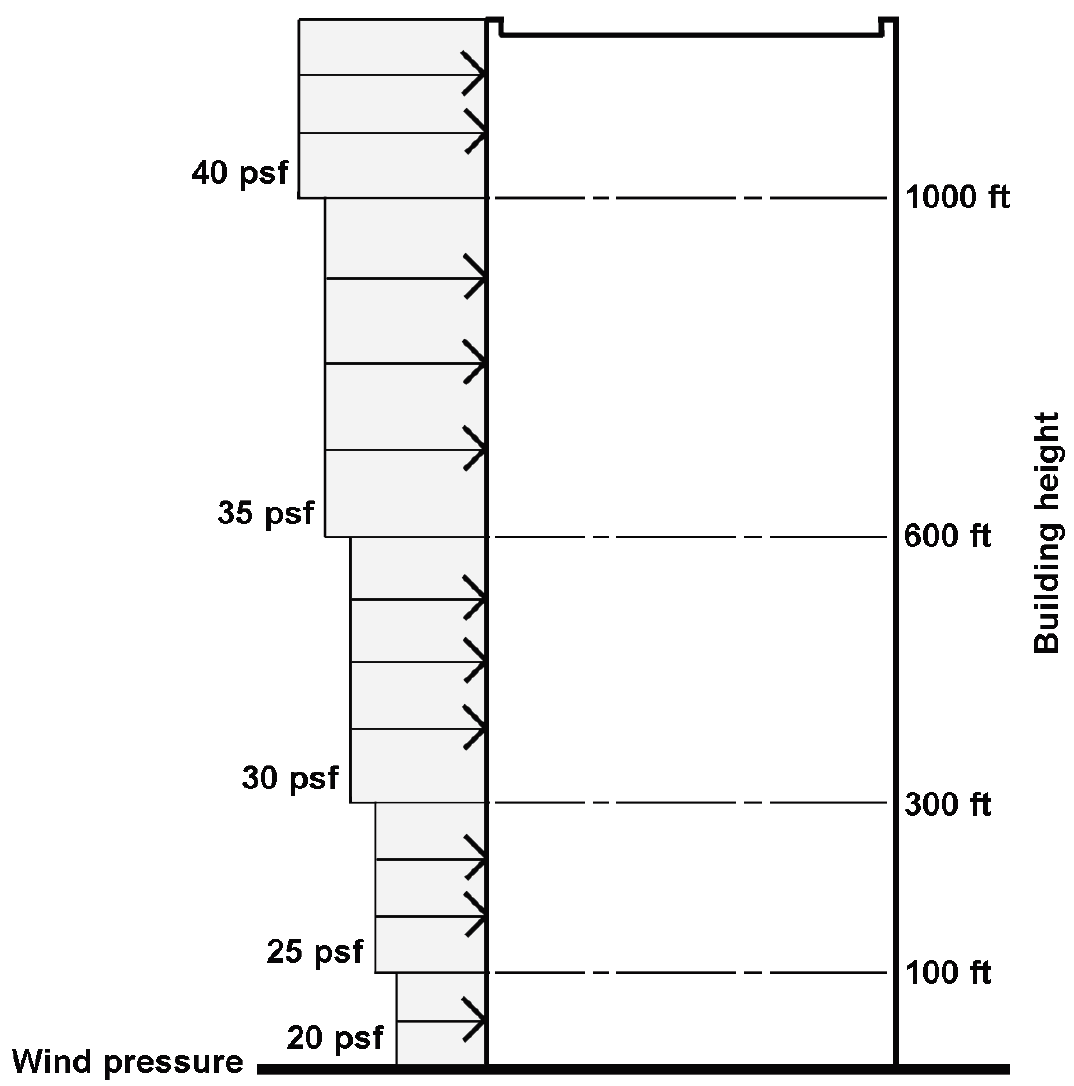
The Building Code of the City of New York historically took the first approach, specifying a 30 psf horizontal wind pressure on the surfaces of buildings over 100 ft tall. This number was actually reduced to 20 psf in the 1930s and 1940s. Then, as buildings grew consistently taller and more data was assembled about wind speed at various elevations above grade, wind pressure began to be modeled as a discontinuous function, increasing from 20 psf below 100 feet to 40 psf above 1000 feet (Figure 2.13).
In contrast to this approach, wind pressure can also be calculated directly from wind speed: the relationship between the velocity or "stagnation" pressure, q, and the basic wind speed, V, is derived from Bernoulli's equation for streamline flow:
where p is the mass density of air. Making some assumptions about air temperature to calculate p, defining qz as the velocity pressure at height z above ground, and converting the units to pounds per square foot (psf) for qz and miles per hour (mph) for V, we get: qz = 0.00256KzKztKdKeV2 (2.6)
where Kz accounts for heights above ground different from the 10 m above ground used to determine nominal wind speeds as well as different "boundary layer" conditions, or exposures, at the site of the structure; Kzt is a factor used only in special cases of increased wind speeds caused by hills, ridges, escarpments, and similar topographic features; the wind directionality factor, Kd , can be taken as 0.85 in most cases and accounts for the fact that the direction of a worst-case wind event may not coincide with the building's weakest aerodynamic profile, although more conservative values for Kd are suggested for chimneys and other similar roof-top structures; and Ke is a ground elevation factor that can be taken conservatively as 1.0 for all buildings, but which — alternatively — can be reduced by as much as 80 percent when the ground level is 6,000 feet or more above sea level (accounting for the impact of reduced air density on velocity pressure). The importance factor, formerly included in this equation to account for relative hazards to life and property associated with various types of occupancies, is now incorporated directly into wind speed maps — that is, it shows up as part of V.
For a building close to sea level with normal occupancy at a height of 10 meters above grade in open terrain, i.e., with Kz = Kd = Kzt = Ke = 1.0, a wind speed of 115 mph corresponds to a velocity pressure equal to:
The external design wind pressure, pe, can be found at any height, and for various environmental and building conditions, by multiplying the velocity pressure, qz, by a series of coefficients corresponding to those conditions:
where qz is the velocity pressure as defined in Equation 2.6; G accounts for height-dependent gustiness; and Cp is a pressure coefficient accounting for variations in pressure and suction on vertical, horizontal and inclined surfaces. Combining Equations 2.6 and 2.8, we get:
where:
pe = the external design wind pressure (psf)
V = the basic wind speed (mph)
Kz = the velocity pressure exposure coefficient
Kd = 0.85 is a wind directionality factor (for use only when computing load combinations)
Kzt = a topography factor (can be taken as 1.0 unless the building is situated on a hill, ridge, escarpment, etc.)
Ke = a ground elevation factor
G = a coefficient accounting for height-dependent gustiness
Cp = a pressure coefficient accounting for variations in pressure and suction on vertical, horizontal and inclined surfaces
Some values for these coefficients — for buildings in various terrains (exposure categories) — are given in Appendix Table A-2.5 (except that wind velocities, V, for various cities and risk categories, are found in Appendix Table A-2.3). The resulting distribution of wind pressures on all exposed surfaces of a generic rectangular building (with a sloped roof) is shown in Figure 2.14.
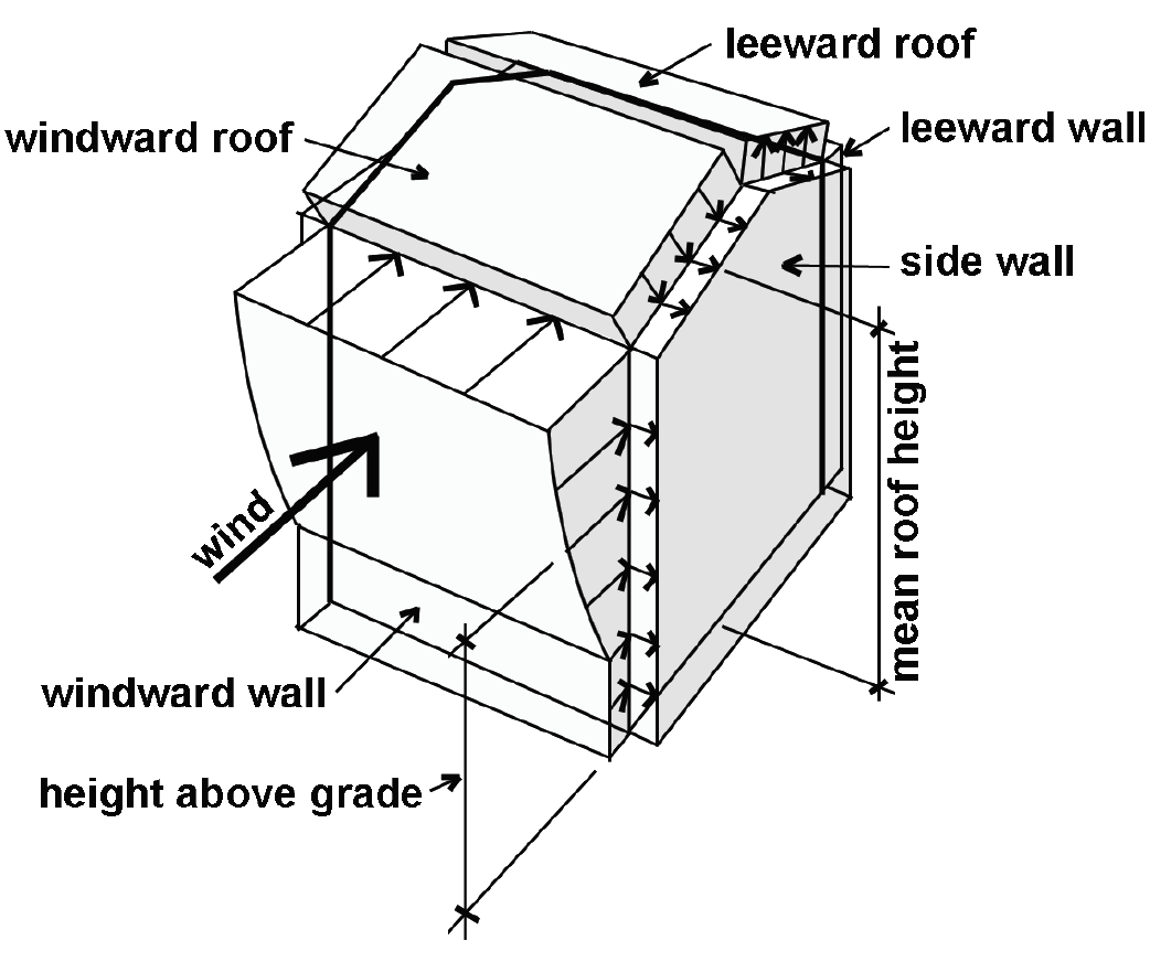
Only on the windward wall of the building does the wind pressure vary with height above ground. On all other surfaces, the coefficient Kz is taken at mean roof height for the entire surface, resulting in a uniform distribution of wind pressure (whereas for the windward wall, the coefficient Kz is taken at the height at which the pressure is being computed). This is consistent with the results of wind tunnel tests, which show a much greater variability (related to height) on the windward wall than on any other surface.
Changes in the building's internal pressure as a result of high winds can increase or decrease the total pressure on portions of a structure's exterior "envelope." This internal pressure, pi, is normally taken as 18% of the roof-height velocity pressure for enclosed buildings, but can be as high as 55% of the roof-height velocity pressure for partially-enclosed buildings The total design pressure, p, is therefore:
The actual behavior of wind is influenced not only by the surface (or boundary layer) conditions of the earth, but also by the geometry of the building. All sorts of turbulent effects occur, especially at building corners, edges, roof eaves, cornices, and ridges. Some of these effects are accounted for by the pressure coefficient Cp, which effectively increases the wind pressure at critical regions of the building envelope. Increasing attention is also being given to localized areas of extremely high pressure, which are averaged into the total design pressures used when considering a structure's "main wind-force resisting system" (MWFRS). These high pressures need to be considered explicitly when examining the forces acting on relatively small surface areas, such as mullions and glazing, plywood sheathing panels, or roofing shingles. Building codes either stipulate higher wind pressures for small surface elements like glass and wall panels, or provide separate "component and cladding" values for the external pressure coefficients and gust response factors.
Since both external and internal pressures can be either positive (i.e., with the direction of force pushing on the building surface), or negative (i.e., with a suction-type force pulling away from the building surface), the total design pressure on any component or cladding element is always increased by the consideration of both external and internal pressures. For certain MWFRS calculations, however, the internal pressures on opposite walls cancel each other so that only external pressures on these walls need to be considered.
As an alternative to the analytic methods described above, three other methods are also permitted: a simplified tabular method for certain buildings no more than 160 ft high, a simplified analytic procedure for enclosed, more-or-less symmetrical low-rise (no more than 60-feet high) buildings; and physical testing of models within wind-tunnels to determine the magnitudes and directions of wind-induced pressures.
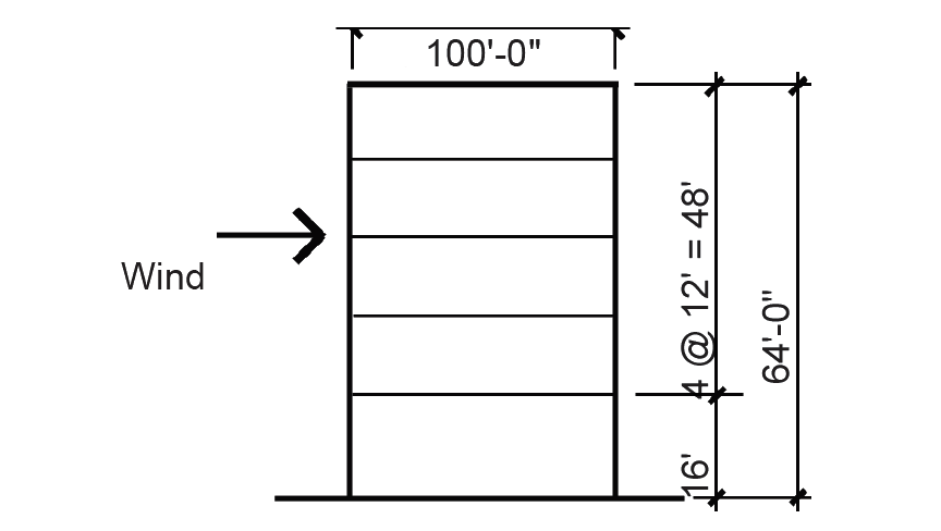
Problem definition. Find the distribution of wind load on the windward and leeward surfaces of a 5-story office building located in the suburbs of Chicago. We will assume typical "suburban" terrain, or Exposure Category B. The wind directionality factor Kd = 0.85 for main wind force resisting systems; and the ground elevation factor, Ke = 1.0. The topography factor, Kzt = 1.0, since no peculiar topographic features are present, and wind speed is found based on a "risk category" of II corresponding to normal occupancy. A typical building section is shown in Figure 2.15. Plan dimensions are 100 ft × 100 ft. Neglect internal pressure.
Solution overview. Find basic wind speed; compute external design wind pressures.
Problem solution
1. From Appendix Table A-2.3, the basic (ultimate) wind speed, V = 115 mph.
2. Windward wall: From Equation 2.9, we find the external design wind pressure:
pe = 0.00256KzKztKdKeGCpV2
where values for Kz , G, and Cp are found in Appendix Table A-2.5 (Kzt, Kd ,and Ke are given in the problem statement). It is convenient to organize the solution in tabular form, as shown below in Table 2.1. The value of Kz at mean roof height (64 ft) is found by interpolation between the value at 60 ft and the value at 70 ft: from which Kz = 0.87. The values for Kzt = Ke = 1.0.
Table 2.1: Calculation of external design windward wall pressure for Example 2.4
| Height | 0.00256 | Kz | Kzt | Kd | Ke | G | Cp | V2 (mph) | pe (psf) |
|---|---|---|---|---|---|---|---|---|---|
| 70 | 0.00256 | 0.89 | 1.0 | 0.85 | 1.0 | 0.85 | 0.8 | 115 × 115 | 17.42 |
| 64 | 0.00256 | 0.87 | 1.0 | 0.85 | 1.0 | 0.85 | 0.8 | 115 × 115 | 17.02 |
| 60 | 0.00256 | 0.85 | 1.0 | 0.85 | 1.0 | 0.85 | 0.8 | 115 × 115 | 16.63 |
| 50 | 0.00256 | 0.81 | 1.0 | 0.85 | 1.0 | 0.85 | 0.8 | 115 × 115 | 15.85 |
| 40 | 0.00256 | 0.76 | 1.0 | 0.85 | 1.0 | 0.85 | 0.8 | 115 × 115 | 14.87 |
| 30 | 0.00256 | 0.70 | 1.0 | 0.85 | 1.0 | 0.85 | 0.8 | 115 × 115 | 13.70 |
| 20 | 0.00256 | 0.62 | 1.0 | 0.85 | 1.0 | 0.85 | 0.8 | 115 × 115 | 12.13 |
| 0 – 15 | 0.00256 | 0.57 | 1.0 | 0.85 | 1.0 | 0.85 | 0.8 | 115 × 115 | 11.153 |
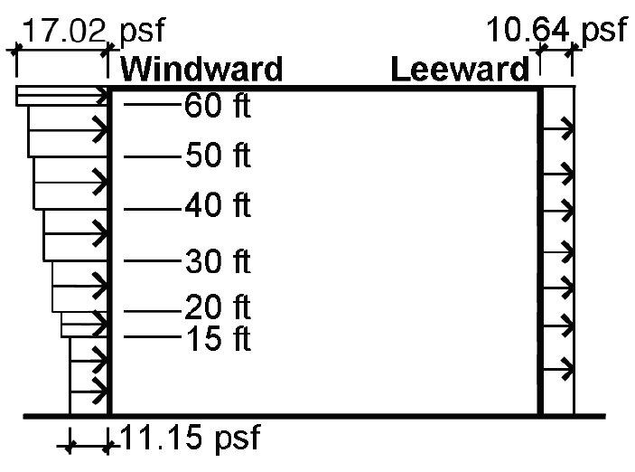
3. Leeward wall: From Equation 2.9, the external design wind pressure for the leeward wall can be found (there is only one value for the entire leeward wall, based on Kz at the mean roof height). From Appendix Table A-2.5, Cp = –0.5 (since the ratio L/B = 100/100 = 1.0); Kz = 0.87 (at mean roof height: see step 2); G = 0.85; Kd = 0.85; and Kzt = Ke = 1.0. The external wind pressure on the leeward side of the building is therefore:
pe = (0.00256)(0.87)(1.0)(1.0)(0.85)(0.85)(–0.5)(1152) = –10.64 psf
The negative sign indicates that this leeward pressure is acting in "suction," pulling away from the leeward surface.
4. The distribution of wind pressure on the building section is shown in Figure 2.16. The direction of the arrows indicate positive pressure (pushing) on the windward side and negative pressure (suction) on the leeward side. Rather than connecting the points at which pressures are computed with straight lines (which would result in triangular stress blocks over the surface of the building), it is common to use the more conservative assumption of constant pressure from level to level, which results in a discontinuous, or stepped, pattern of wind pressure, as shown in Figure 2.16.
When computing the magnitude of wind loads that must be resisted by a building's lateral-force-resisting system, internal pressures can be neglected (as they act in opposite directions on the two interior faces of the building, canceling out), leaving only the windward and leeward pressures to be considered for each orthogonal plan direction.
A building riding an earthquake is like a cowboy riding a bull in a rodeo: as the ground moves in a complex and dynamic pattern of horizontal and vertical displacements, the building sways back and forth like an inverted pendulum. The horizontal components of this dynamic ground motion, combined with the inertial tendencies of the building, effectively subject the building structure to lateral forces that are proportional to its weight. In fact, the earliest seismic codes related these seismic forces, F, to building weight, W, with a single coefficient:
where C was taken as 0.1.
What this simple equation doesn't consider are the effects of the building's geometry, stiffness and ductility, as well as the characteristics of the soil, on the magnitude and distribution of these equivalent static forces. In particular, the building's fundamental period of vibration, related to its height and type of construction, is a critical factor. For example, the periods of short, stiff buildings tend to be similar to the periodic variation in ground acceleration characteristic of seismic motion, causing a dynamic amplification of the forces acting on those buildings. This is not the case with tall, slender buildings having periods of vibration substantially longer than those associated with the ground motion. For this reason, tall flexible buildings tend to perform well (structurally) in earthquakes, compared to short, squat and stiff buildings.
But stiffness can also be beneficial since the large deformations associated with flexible buildings tend to cause substantial nonstructural damage. The "ideal" earthquake-resistant structure must therefore balance the two contradictory imperatives of stiffness and flexibility.
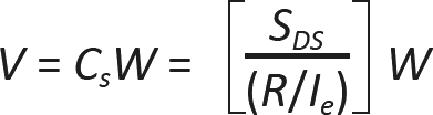
In modern building codes, the force F has been replaced with a "design base shear," V, equal to the total lateral seismic force assumed to act on the building. Additionally, the single coefficient relating this shear force to the building's weight ("seismic dead load") has been replaced by a series of coefficients, each corresponding to a particular characteristic of the building or site that affects the building's response to ground motion. Thus, the base shear can be related to the building's weight with the following coefficients, using an "equivalent lateral force procedure" for seismic design:
where:
V = the design base shear
Cs = the seismic response coefficient equal to SDS/(R/Ie)
W = the effective seismic weight (including dead load, permanent equipment, a percentage of storage and warehouse live loads, partition loads, and certain snow loads)
SDS = the design elastic response acceleration at short periods
R = a response modification factor (relating the building's lateral-force-resisting system to its performance under seismic loads)
Ie = the seismic importance factor (with somewhat different values than the equivalent factors for wind or snow)
The coefficient Cs has upper and lower bounds that are described in Appendix Table A-2.6 part H, so it will only correspond to the value defined in Equation 2.12 when it falls between the two bounding values. The response modification factor, R, is assigned to specific lateral-force-resisting systems — not all of which can be used in every seismic region or for every type of occupancy; Appendix Table A-2.6, part D, indicates which structural systems are either not permitted, or limited in height, within specific seismic design categories.
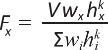
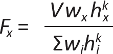
To approximate the structural effects that seismic ground motion produces at various story heights, seismic forces, Fx, are assigned to each level of the building structure in proportion to their weight times height (or height raised to a power no greater than two) above grade:
where:
V = the design base shear, as defined above in Equation 2.12
wi and wx = the portions of weight W at, or assigned to, a given level, i or x
hi and hx = the heights from the building's base to level i or x
k = 1 for periods ≤ 0.5s and 2 for periods ≥ 2.5s (with linear interpolation permitted for periods between 0.5s and 2.5s) and accounts for the more complex effect of longer periods of vibration (defined in Appendix Table A-2.6, part E) on the distribution of forces
The Σ symbol in Equation 2.13 indicates the sum of the product of (wihik) for i ranging from 1 to n, where n is the number of levels at which seismic forces are applied.
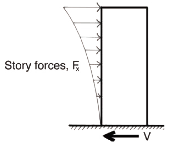
A typical distribution of lateral seismic forces resulting from the application of this equation is shown in Figure 2.17. It can be seen that Equation 2.13 for Fx guarantees that these story forces are in equilibrium with the design base shear, V.
By considering both a building's occupancy category (see Appendix Table A-2.6, part F ) and the expected ground motion at the building's site, a Seismic Design Category, or SDC, can be determined. Criteria for a building's SDC are found in Appendix Table A-2.6, part G. For structures that are in the lowest-risk SDC A, it is not necessary to consider the design of nonstructural components for seismic resistance. On the other hand, for the highest-risk SDCs C, D, E, and F, increased scrutiny is required: issues of slope instability, liquifaction, settlement, surface displacement, and — for SDCs D, E, and F only — lateral pressure on basements must be considered. Such issues are beyond the scope of this chapter. Buildings with the most extreme SDCs E and F are not permitted where the ground surface might be ruptured by a known active fault.
Building codes require that larger seismic forces be used for the design of individual building elements, and for the design of floor "diaphragms." The rationale for the separate calculation of these forces is similar to the logic behind the calculation of larger "component and cladding" loads in wind design: because the actual distribution of seismic forces is nonuniform, complex, and constantly changing, the average force expected to act upon the entire lateral-force-resisting structural system is less than the maximum force expected to occur at any one level, or upon any one building element.
While we tend to think of seismic forces as acting in the horizontal direction, there are also vertical forces associated with earthquake-induced ground motion. For any structural element, the effects of the horizontal story forces, or Eh, must be combined with the effects of these vertical ground motions, which can be approximated as Ev = 0.2SDSD. In this equation, values for SDS, the design elastic response acceleration at short period described above, can be found in Appendix Table A-2.6, part C; while D represents the effect of the dead load on the particular structural element being analyzed. Dead loads are taken as positive when acting downward, and therefore the same sign convention applies to the effect of the vertical component of seismic ground motion, Ev. The effects of both horizontal and (downward-acting) vertical earthquake forces must be added together when considering the overall effect when earthquake loads, E, are used in combination with live loads, dead loads, and snow loads. On the other hand, the vertical component of earthquake loads must be subtracted from the horizontal component when only the effects of dead load and earthquake load are considered. This is because the worst-case scenario represented by this load combination is triggered by uplift, i.e., by a negative value of Ev combined with a reduced value of the dead load effect, D. Load combinations are discussed in more detail later in this chapter. In any case, Ev can be ignored for buildings in Seismic Design Category B.
The determination of the effect that horizontal story forces have on any structural element, i.e., the determination of Eh, presumes that the structure has adequate redundancy to avoid failure due to extreme torsional irregularity or other conditions that might reduce the shear capacity at any particular story level. Where this redundancy cannot be taken for granted — in particular for structures in Seismic Design Categories D, E, and F — Eh must be multiplied by a redundancy factor, ρ = 1.3. This redundancy factor can be eliminated, i.e, ρ can be taken as 1.0, for structures in Seismic Design Category D without extreme torsional irregularities; or, for stories in Seismic Design Categories E and F — already prohibited from having extreme torsional irregularities — where no more than 35% of the base shear, V, must be resisted (typically only for the top stories of tall buildings).
The "equivalent lateral force analysis" method described above is but one of several alternate procedures developed for seismic force calculations. In addition to a "simplified analysis" method for most non-hazardous and nonessential low-rise structures, more sophisticated alternate methods have been developed that can be used for any structure in any seismic region. These methods include modal response spectrum analysis as well as both linear and nonlinear response history analysis, all beyond the scope of this text.
Whatever the method of analysis, designers in seismically-active regions should carefully consider the structural ramifications of their "architectural" design decisions, and provide for ductile and continuous load paths from roof to foundation. Following are some guidelines:
Avoid "irregularities" in plan and section. In section, these irregularities include soft stories and weak stories that are significantly less stiff or less strong than the stories above; and geometric irregularities and discontinuities (offsets) within the structure. Plan irregularities include asymmetries, reentrant corners, discontinuities and offsets that can result in twisting of the structure (leading to additional torsional stresses) and other stress amplifications. Buildings articulated as multiple masses can be either literally separated (in which case the distance between building masses must be greater than the maximum anticipated lateral drift, or movement), or structurally integrated (in which case the plan and/or sectional irregularities must be taken into account).
Provide tie-downs and anchors for all structural elements, even those that seem secured by the force of gravity: the vertical component of seismic ground acceleration can "lift" buildings off their foundations, roofs off of walls, and walls off of framing elements unless they are explicitly and continuously interconnected. Nonstructural items such as suspended ceilings, mechanical and plumbing equipment must also be adequately secured to the structural frame.
The explicit connection of all structural elements is also necessary for buildings subjected to high wind loads, since uplift and overturning moments due to wind loads can pull apart connections designed on the basis of gravity loads only. But unlike seismic forces, which are triggered by the inertial mass of all objects and elements within the building, wind pressures act primarily on the exposed surfaces of buildings, so that the stability of interior nonstructural elements is not as much of a concern.
Avoid unreinforced masonry or other stiff and brittle structural systems. Ductile framing systems can deform inelastically, absorbing large quantities of energy without fracturing.
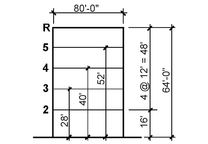
Problem definition. Find the distribution of seismic story loads on a 5-story office building located in San Francisco. Plan dimensions are 60 ft × 80 ft; assume that an "effective seismic weight" of 75 psf can be used for all story levels above grade, including the roof (primarily due to the dead load). The structure is a steel special moment-resisting frame and is built upon dense soil. The typical building section is shown in Figure 2.18.
Solution overview. Find the effective seismic weight, W and the seismic response coefficient, Cs; compute the base shear, V, and the story forces, Fx.
Problem solution
1. Find w: The effective seismic weight for each story is the unit weight times the floor area = 75(60 × 80) = 360,000 lb = 360 kips per floor; the total weight, W, for the entire building (floors 2 – 5 plus roof) is therefore 5 × 360 = 1800 kips.
2. Find V:
a. From Appendix Table A-2.3, find Ss, S1 (maximum considered earthquake ground motion at short and long periods, respectively), and TL (long-period transition period) for San Francisco: Ss = 1.50; S1 = 0.60; TL = 12.
b. From Appendix Table A-2.6 parts A and B, find site coefficients Fa and Fv: using dense soil (corresponding to Site Class C) and the values of Ss and S1 found in step a, we find that Fa = 1.2 and Fv = 1.4.
c. From Appendix Table A-2.6 part C, find the design elastic response accelerations: SDS = (2/3)(FaSs) = (2/3)(1.2)(1.5) = 1.2; SD1 = (2/3)(FvS1) = (2/3)(1.4)(0.60) = 0.56.
d. From Appendix Table A-2.6 part D, the response modification factor, R = 8 (for special steel moment frames). There are no height limits or other restrictions for this structural system category; otherwise, it would be necessary to check which seismic design category the building falls under, from Appendix Table A-2.6 part G.
e. From Appendix Table A-2.6 part E, the fundamental period of vibration, T, can be taken as CThnx = 0.028(640.8) = 0.78 second, where hn = 64 ft is the building height; and the values used for CT and x, taken from Appendix Table A-2.6 part E, correspond to steel moment-resisting frames.
f. From Appendix Table A-2.6 part F, the importance factor, Ie equals 1.0 for ordinary buildings.
g. It is now possible to find the seismic response factor, Cs. From Appendix Table A-2.6 part H, the provisional value for Cs = SDS /(R/Ie) = 1.2/(8/1.0) = 0.15. However, this must be checked against the upper and lower limits shown in the table: since S1 = 0.60 ≥ 0.6 and T = 0.78 < TL = 12, the lower limit for Cs is the greater value of 0.044SDSIe = 0.044(1.2 × 1.0) = 0.0528, or 0.01; or 0.5S1 /(R/Ie) = 0.5(0.60)/(8/1.0) = 0.0375; i.e., the lower limit is 0.0528 and the upper limit is Cs = SD1/(TR/Ie) = 0.56/(0.78 × 8/1.0) = 0.090. The upper limit governs in this case, so we use Cs = 0.090.
h. From Equation 2.12, the base shear, V = CsW = 0.090(1800) = 162 kips.
3. From Equation 2.13, the story forces can be determined as follows:
In this equation, since the period, T = 0.78 seconds, is between 0.5 and 2.5, and the limiting values of the exponent, k, are set at 1.0 for T ≤ 0.5 and 2.0 for T ≥ 2.5, our value of k is found by linear interpolation:
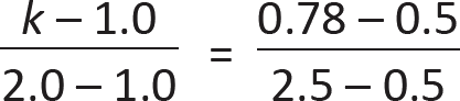
from which k = 1.14. The seismic weight at each story, wi = 360 kips (see step 1), and the various story heights can be most easily computed in tabular form (as shown below in Table 2.2).
Table 2.2: Calculation of story forces for Example 2.5
| Story level | Story height, hx (ft) | hx1.14 | Fx = 0.476hx1.14 (kips) |
|---|---|---|---|
| Roof | 64 | 114.56 | 54.55 |
| 5 | 52 | 90.42 | 43.05 |
| 4 | 40 | 67.04 | 31.92 |
| 3 | 28 | 44.64 | 21.26 |
| 2 | 16 | 23.59 | 11.23 |
| Sum of story forces, Fx = base shear V = | 162 | ||
Once the values for hx1.14 have been determined for each story level, Equation 2.13 can be rewritten as:
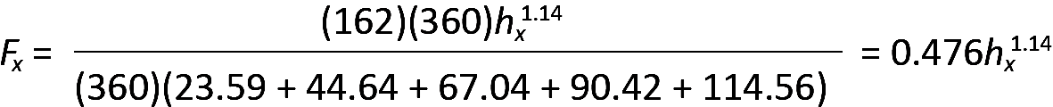
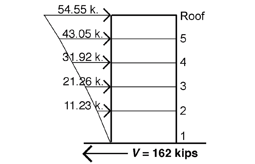
and values for Fx = 0.476hx1.14 can then be added to the table. Finally, their distribution on the building can be sketched, as shown in Figure 2.19. The sum of all the story forces, Fx, equals the design base shear, V, as it must to maintain horizontal equilibrium.
© 2020 Jonathan Ochshorn; all rights reserved. This section first posted November 15, 2020; last updated November 15, 2020.